Introduction to Local Interpretable Model-Agnostic Explanations (LIME)#
Theoretical Background#
Local Interpretable Model-Agnostic Explanations is a model-agnostic method, which means that it is not restricted to a certain model type, and it is a local method, which means that it only provides explanations for individual samples. LIME was introduced in 2016 by Rubiero et. al.
For a short video introduction to LIME, click below:
To summarize, LIME, an abbreviation for “local interpretable model agnostic explanations” is an approach that tries to deliver explanations for individual samples. It works by constructing an interpretable surrogate model (like a linear regression model) to approximate predictions of a more complex model in the neighborhood of a given sample.
LIME for Image Classification#
The paper Garreau et. al. provides a detailed explanation of LIME for images, but let’s summarize the main concepts.
On images, LIME creates perturbations by altering regions of the image, constructs a dataset with interpretable features for a surrogate model using these perturbed images, and measures model prediction changes using a glassbox model (here a linear model) to highlight the most influential regions.
How do we create the image perturbation?#
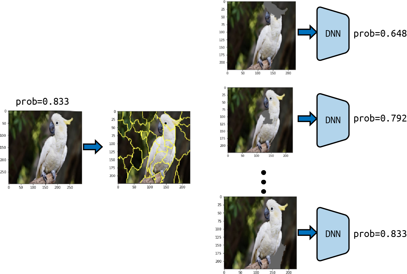
LIME segments the image into sections known as superpixels, breaking it down into $d$ subregions referred to as interpretable fearures. The default segmentation algorithm of LIME to produce this superpixels is the quickshift algorithm by Vedaldi et. al. However, you can choose a different segmentation algorithm available at scikit-image. LIME introduces perturbations to these interpretable components by modifying pixel values within each superpixel region, typically turning them gray or replacing them with the mean of all pixels in the superpixel. Each perturbed instance is then fed into the model to generate new predictions for the originally predicted class. These predictions will be the labels for the new dataset. This dataset is utilized to train LIME’s linear model, helping assess the contribution of each interpretable component to the original prediction.
In the image (source) below, we can see an example of the original image on the left and an overlay of the superpixels (yellow) in the middle. On the right, we can see some examples of perturbed images passed to the inference algorithm to make new predictions.
How do we create the dataset for the surrogate model?#
LIME creates the dataset from the $n$ perturbed images. For each newly generated example $x_i$, the superpixels are randomly switched on and off, and this information is encoded in a vector $z_i ∈ {0, 1}^d$, where each coordinate of $z_i$ corresponds to the activation \(z_\mathrm{i,j} = 1\) or inactivation \(z_{i,j} = 0\) of superpixel $j$. We call the $z_i$ the interpretable features. These perturbations are just simple binary representations of the image indicating the “presence” or “absence” of each superpixel region. Since we care about the perturbations closest to the original image, those examples with the most superpixels present are weighted more than examples with more superpixels absent. This proximity can be measured using any distance metric for images.
How do we measure the change in the model prediction?#
In the next step, LIME builds a surrogate model with the interpretable features $z_i$ as input and the predicted outcomes \(y_i:= f(x_i)\) as responses, i.e., labels. The linear model is represented as:
Here, \(\hat{y}_i\) is the outcome predicted by the surrogate model for the $i$-th perturbed instance, \(z_{i,j}\) is the $j$-th interpretable feature, and \(\epsilon_i\) is the prediction error with respect to the actual label $y_i$. In the default implementation, LIME obtains this linear model using a (weighted) ridge regression. The final step involves displaying the superpixels associated with the top positive coefficients of $beta$.
References#
Original LIME paper: Ribeiro, M. T., Singh, S., & Guestrin, C. “Why should i trust you?” Explaining the predictions of any classifier. ACM. 2016.
LIME for images: Garreau, D., & Mardaoui, D. What does LIME really see in images? PMLR. 2021
Quickshift segmentation algorithm: Vedaldi, A., & Soatto, S. Quick shift and kernel methods for mode seeking. ECCV. 2008.
XAI Book: Molnar, C. Interpretable Machine Learning: A Guide for Making Black Box Models Explainable. Lulu.com. 2022.